39 excel donut chart labels
Labels for pie and doughnut charts - Support Center To format labels for pie and doughnut charts: 1. Select your chart or a single slice. Turn the slider on to Show Label. 2. Use the sliders to choose whether to include Name, Value, and Percent. 3. Use the Precision setting allows you to determine how many digits display for numeric values. 4. Fix label position in doughnut chart? | MrExcel Message Board Turn off data labels. Insert a Text box in to the middle of the donut, select the edge of the text box and in the formula bar hit = then select the cell that contains the progress figure. You can format this to however you want it, it will update and it won't move. Click to expand... Oh wow! I always thought text-boxes were just text-boxes.
How to Make a Doughnut Chart in Excel | EdrawMax Online How to Make a Doughnut Chart in EdrawMax Step 1: Select Chart Type When you open a new drawing page in EdrawMax, go to Insert tab, click Chart or press Ctrl + Alt + R directly to open the Insert Chart window so that you can choose the desired chart type.

Excel donut chart labels
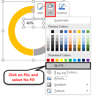
Add / Move Data Labels in Charts - Excel & Google Sheets Adding and Moving Data Labels in Google Sheets Starting with your Data. We'll start with the same dataset that we went over in Excel to review how to add and move data labels to charts. Add and Move Data Labels in Google Sheets. Double Click Chart; Select Customize under Chart Editor; Select Series . 4. Check Data Labels. 5. Curved labels in Excel doughnut chart - Microsoft Community All I've seen is that you can display labels in straight lines. You can angle them, rotate them, invert them, but not curve them. You can even make them "dynamic", but no mention of curved text. The simple reality is that in terms of presentation, excel is primitive. . This article shows the label options in 2016, no mention of curves How to create a creative multi-layer Doughnut Chart in Excel By default, all doughnut chart layers have a borderline. As this border line is only disrupting the look, you should remove it for all borders first. After that, select the outer layer of the second (also second biggest) data point and set the fill to No fill. For the third data point we apply the same technique to the two outer layers, and so on.
Excel donut chart labels. Create Radial Bar Chart in Excel - Step by step Tutorial 25.06.2022 · This unique Excel graph is useful for sales presentations and reports. First, let us see the initial data set! Then, we’ll compare five products. Step 1: Check this range below! You can include the Product Name and Sales fields. The first field is placed in column ‘B’. The second field is in column ‘C’. Using this data set, we’ll ... How to Create Doughnut Excel Chart? - WallStreetMojo doughnut chart is a type of chart in excel whose function of visualization is just similar to pie charts, the categories represented in this chart are parts and together they represent the whole data in the chart, only the data which are in rows or columns only can be used in creating a doughnut chart in excel, however it is advised to use this … Everything About Donut Charts [+ Examples] | EdrawMax Unlike other charts, donut charts only have two types: a simple donut chart and an exploded donut chart. Let's take a look at how they are different from one another. • Donut Chart. This type is the primary type of donut chart. It consists of a ring that displays the data. If the data labels consist of percentages, each round will depict 100%. Interactive Donut Chart - Beat Excel! Now select and copy the first gray area in Sheet 2 that includes blue donut part and paste it as a linked picture to cell B2 of Sheet 1. Click on this picture and type =Chart inside the formula bar. Do the same with the label but this time place it in the middle of the gray area in Sheet 1. While on Sheet 1, insert a donut chart as shown below.
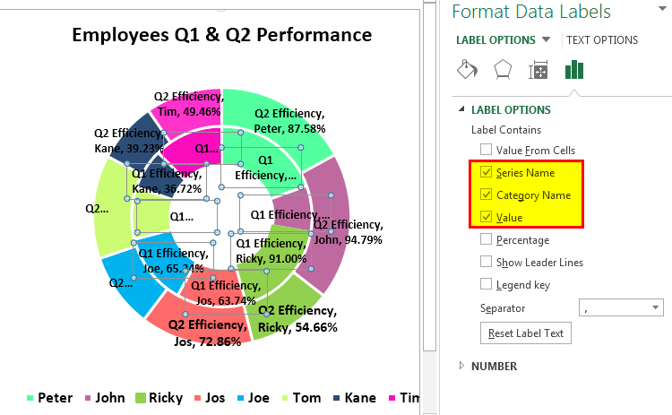
Excel 2007 Doughnut chart Label Bug E.g. Series 1 with A, B and C, Series 2 with A1, A2, B1, B2, B3, C1 and C2. Either the Series 1 gets the labels A1, A2, B1 from series 2. Or, if added in the other order, then Series 2 getes the labels A, B, C for the 1st three data points and no labels for the remaining points. Value and Percentage in the data labels is working well! How to add leader lines to doughnut chart in Excel? Select data and click Insert > Other Charts > Doughnut. In Excel 2013, click Insert > Insert Pie or Doughnut Chart > Doughnut. 2. Select your original data again, and copy it by pressing Ctrl + C simultaneously, and then click at the inserted doughnut chart, then go to click Home > Paste > Paste Special. See screenshot: 3. Donut, column, and bar chart dashboard - templates.office.com Add this dashboard including donut, column, and bar charts to any slideshow. This is an accessible template. Add this dashboard including donut, column, and bar charts to any slideshow. ... Excel Wedding budget template Excel USA chart dashboard PowerPoint Baby growth chart Excel ... Labels. Learning. Letters. Lists. Logs. Maps. Memos. Menus ... chandoo.org › wp › change-data-labels-in-chartsHow to Change Excel Chart Data Labels to Custom Values? May 05, 2010 · First add data labels to the chart (Layout Ribbon > Data Labels) Define the new data label values in a bunch of cells, like this: Now, click on any data label. This will select “all” data labels. Now click once again. At this point excel will select only one data label.
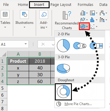
How to create doughnut chart in Excel? - ExtendOffice In Excel 2013, click Insert > Insert Pie or Doughnut Chart > Doughnut. See screenshot: 2. Then a doughnut chart is inserted in your worksheet. Now you can right click at all series and select Add Data Labels from the context menu to add the data labels. See screenshots: Now a simple doughnut chart is created. Pie chart maker | Create a pie graph online - RapidTables.com Use 2 underlines '__' for 1 underline in data labels: 'name__1' will be viewed as 'name_1' Pie chart. Pie chart is circle divided to slices. Each slice represents a numerical value and has slice size proportional to the value. Pie chart types. Circle chart: this is a regular pie chart. 3D pie chart: the chart has 3D look. donut chart labels - Microsoft Community Click the chart. On the Format tab, in the Size group, enter the size that you want in the Shape Height and Shape Width box. Tip For our doughnut chart, we set the shape height to 4" and the shape width to 5.5". To change the size of the doughnut hole, do the following: Question: labels in an Excel doughnut chart - Microsoft Tech Community Open your Excel document and click on your chart. In the upper bar you will find the "Diagram Tools". Click on the "Design" tab. In the "Data" group, click the "Select data" button. In the right window you will find the "Horizontal axis label". Click on "Edit". Now enter your desired names or values for the legend.
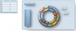
Interactive Donut Chart - Beat Excel!
Excel - techcommunity.microsoft.com 11.03.2021 · Your community for how-to discussions and sharing best practices on Microsoft Excel. If you’re looking for technical support, please visit Microsoft
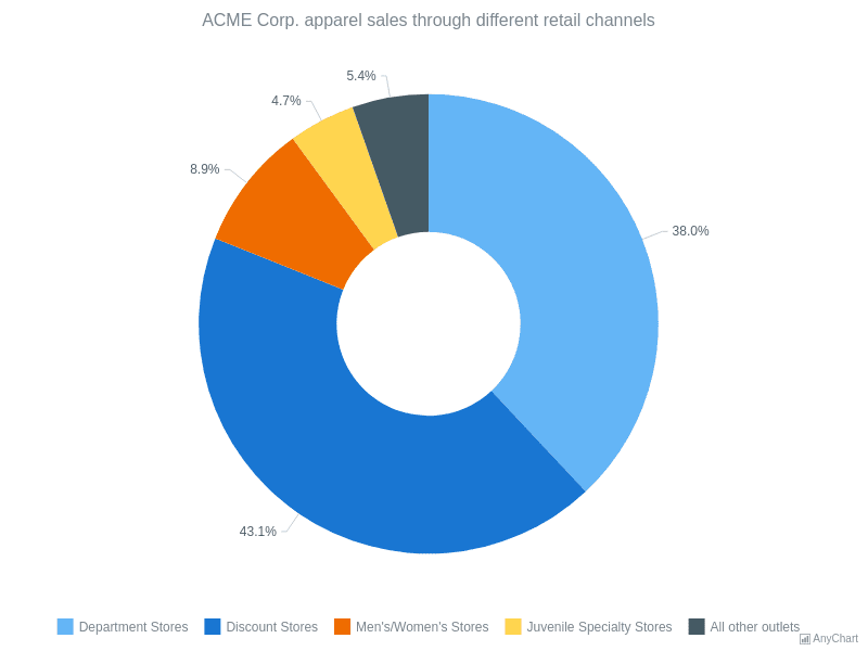
Pie and Donut Charts | AnyChart Gallery
Format Bar Chart in Power BI - Tutorial Gateway To enable or format Power BI bar chart data labels, please toggle Data labels option to On. Let me change the Color to Green, Display Units from Auto to Thousands, Font family to DIN, Text Size to 10, and Background color to Black with 90% transparency . Format Bar Chart in Power BI Plot Area. You can add Images as the Background of a Bar Chart using this Plot Area …
Excel Donut Chart Template
excel - Positioning labels on a donut-chart - Stack Overflow The option to place the labels outside the chart is not available on the doughnut chart options: like they do on a pie chart: However, you could perform a trick using a pie chart and a white circle to make it look like a doughnut by doing the following: Sub AddCircle () 'Get chart size and position: Dim CH01 As Chart: Set CH01 = ThisWorkbook ...

Pie Chart Templates
Donut/Doughnut Chart - Multiple Series - Microsoft Tech Community I have created a doughnut chart with multiple series (represented by multiple rings - see charts below). Each ring is divided into 6, the colour of which corresponds to one of three options (yes, maybe and no). I therefore want the colour of the chart to represent this clearly (green, yellow and red...
Doughnut Chart in Excel | How to Create Doughnut Chart in Excel?
donut chart don't show all labels - Microsoft Power BI Community Because I cannot figure out why sometimes labels for the smaller values are shown and labels for larger values are not shown. e.g. in the below charts example Chart 1 all values are shown. Chart 2 I have added Germany. But the label for Columbia (2.13%) is not shown but smaller value Angola (0.92%) is shown. Message 22 of 30.
Doughnut Chart in Excel | How to Create Doughnut Excel Chart?
templates.office.com › en-au › Simple-Gantt-Chart-TMSimple Gantt Chart - templates.office.com Create a project schedule and track your progress with this accessible Gantt chart template in Excel. The professional-looking Gantt chart is provided by Vertex42.com, a leading designer of Excel spreadsheets. The Excel Gantt chart template breaks down a project by phase and task, noting who’s responsible, task start and end date, and percent completed. Share the Gantt chart in Excel with ...

How to create doughnut chart in Excel?
› charts › progProgress Doughnut Chart with Conditional Formatting in Excel The entire chart will be shaded with the progress complete color, and we can display the progress percentage in the label to show that it is greater than 100%. Step 2 - Insert the Doughnut Chart With the data range set up, we can now insert the doughnut chart from the Insert tab on the Ribbon. The Doughnut Chart is in the Pie Chart drop-down menu.
Doughnut Chart in Excel | How to Create Doughnut Chart in Excel?
How to Change Excel Chart Data Labels to Custom Values? 05.05.2010 · First add data labels to the chart (Layout Ribbon > Data Labels) Define the new data label values in a bunch of cells, like this: Now, click on any data label. This will select “all” data labels. Now click once again. At this point excel will select only one data label.
Chart Busters: Fix the Heat Map Donut Chart - Peltier Tech Blog
Curve Text in Doughnut chart - Excel Help Forum Re: Curve Text in Doughnut chart. You can link WordArt to a cell using a formula. Just select the shape, click into the formula bar, type = and then select the cell and press Enter. Please remember to mark your thread 'Solved' when appropriate.

34 How To Label A Pie Chart - Labels Database 2020
How to Create a Double Doughnut Chart in Excel - Statology Step 3: Add a layer to create a double doughnut chart. Right click on the doughnut chart and click Select Data. In the new window that pops up, click Add to add a new data series. For Series values, type in the range of values fpr Quarter 2 revenue: Click OK.
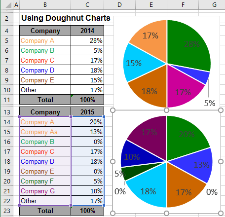
Using Pie Charts and Doughnut Charts in Excel
Show Months & Years in Charts without Cluttering - Chandoo.org 17.11.2010 · So you can just have Product Group & Product Name in 2 columns and when you make a chart, excel groups the labels in axis. 2. Further reduce clutter by unchecking Multi Level Category Labels option. You can make the chart even more crispier by removing lines separating month names. To do this select the axis, press CTRL + 1 (opens format dialog ...

How to Create a Double Doughnut Chart in Excel - Statology
How to Create Doughnut Chart in Excel? - EDUCBA Now we will create a doughnut chart as similar to the previous single doughnut chart. Select the data alone without headers, as shown in the below image. Click on the Insert menu. Go to charts select the PIE chart drop-down menu. From Dropdown, select the doughnut symbol. Then the below chart will appear on the screen with two doughnut rings.
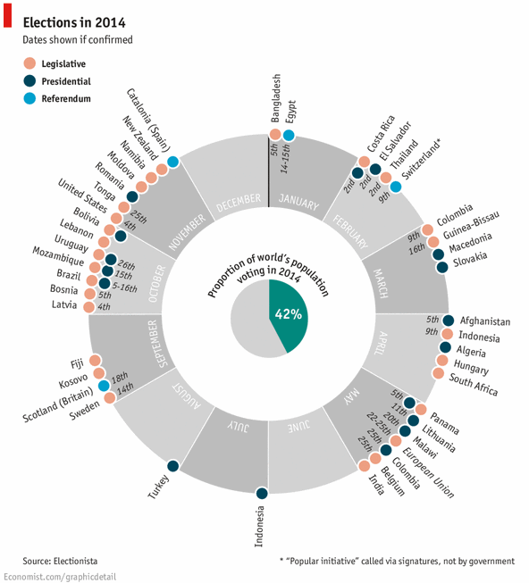
42% of the world goes to polls around a pie chart – Like it or hate it? | Chandoo.org - Learn ...
Excel Doughnut chart with leader lines - teylyn Step 1 - doughnut chart with data labels Step 2 -Add the same data series as a pie chart Next, select the data again, categories and values. Copy the data, then click the chart and use the Paste Special command. Specify that the data is a new series and hit OK. You will see the new data series as an outer ring on the doughnut chart.

Doughnut Chart in Excel - GeeksforGeeks
Free Pie Chart Maker - Make Your Own Pie Chart | Visme Create pie charts with our online pie chart maker. Import Excel data or sync to live data with our pie chart maker. Add several data points, data labels to each slice of pie. Chosen by brands large and small. Our pie chart maker is used by over 14,209,854 marketers, communicators, executives and educators from over 120 countries that include: EASY TO EDIT Pie Chart …

Interactive Donut Chart - Beat Excel!
Excel Charts - Doughnut Chart - Tutorials Point Step 2 − Select the data. Step 3 − On the INSERT tab, in the Charts group, click the Pie chart icon on the Ribbon. It is used to insert a Doughnut chart also. You will see the different types of Doughnut charts available. Step 4 − Point your mouse on the Doughnut icon. A preview of that chart type will be shown on the worksheet.

How to add leader lines to doughnut chart in Excel?
exceldashboardschool.com › radial-bar-chartCreate Radial Bar Chart in Excel - Step by step Tutorial Jun 25, 2022 · This unique Excel graph is useful for sales presentations and reports. First, let us see the initial data set! Then, we’ll compare five products. Step 1: Check this range below! You can include the Product Name and Sales fields. The first field is placed in column ‘B’. The second field is in column ‘C’. Using this data set, we’ll ...
Donut Chart Template for PowerPoint - SlideModel
How to make doughnut chart with outside end labels? - Simple Excel VBA ... In the doughnut type charts Excel gives You no option to change the position of data label. The only setting is to have them inside the chart.
Post a Comment for "39 excel donut chart labels"