43 how to add chart labels in excel
How to Add Axis Label to Chart in Excel - Sheetaki Method 1: By Using the Chart Toolbar. Select the chart that you want to add an axis label. Next, head over to the Chart tab. Click on the Axis Titles. Navigate through Primary Horizontal Axis Title > Title Below Axis. An Edit Title dialog box will appear. In this case, we will input "Month" as the horizontal axis label. Next, click OK. You ... How to Add Labels to Scatterplot Points in Excel - Statology Step 3: Add Labels to Points. Next, click anywhere on the chart until a green plus (+) sign appears in the top right corner. Then click Data Labels, then click More Options…. In the Format Data Labels window that appears on the right of the screen, uncheck the box next to Y Value and check the box next to Value From Cells.
How do I change the X-axis labels in Excel? - Vivu.tv How To Label Axis In Excel? Click the chart, and then click the Chart Design tab. Click Add Chart Element > Axis Titles, and then choose an axis title option. Type the text in the Axis Title box. To format the title, select the text in the title box, and then on the Home tab, under Font, select the formatting that you want.

How to add chart labels in excel
How to Create a Waterfall Chart in Excel - SpreadsheetDaddy 1. Start by selecting the data you need for your chart ( A1:B5 ). 2. Open the Insert tab. 3. Go to the Charts section and select the dropdown with the Waterfall chart option. 4. Choose the Waterfall chart. And just like that, you have your waterfall chart. How to Apply a Filter to a Chart in Microsoft Excel Go to the Home tab, click the Sort & Filter drop-down arrow in the ribbon, and choose "Filter.". Click the arrow at the top of the column for the chart data you want to filter. Use the Filter section of the pop-up box to filter by color, condition, or value. When you finish, click "Apply Filter" or check the box for Auto Apply to see ... Add or remove data labels in a chart - Microsoft Support
How to add chart labels in excel. EOF How to add data labels in excel to graph or chart (Step-by-Step) Add data labels to a chart. 1. Select a data series or a graph. After picking the series, click the data point you want to label. 2. Click Add Chart Element Chart Elements button > Data Labels in the upper right corner, close to the chart. 3. Click the arrow and select an option to modify the location. 4. How to Add Leader Lines in Excel? - GeeksforGeeks Step 1: Select a range of cells for which you want to make a line chart. Step 2: Go to Insert Tab and select Recommended Charts. A dialogue box name Insert Chart appears. Step 3: Click on All Charts and select Line. Click Ok. Step 4: A line chart is embedded in the worksheet. Step 5: Go to Chart Design Tab and select Add Chart Element . Excel: How to Create a Bubble Chart with Labels - Statology To add labels to the bubble chart, click anywhere on the chart and then click the green plus "+" sign in the top right corner. Then click the arrow next to Data Labels and then click More Options in the dropdown menu: In the panel that appears on the right side of the screen, check the box next to Value From Cells within the Label Options ...
How to add text labels on Excel scatter chart axis - Data Cornering Here is the data that I would like to display in the Excel scatter chart. In addition, I would like to add custom labels on Excel scatter chart x-axis with each person's name. Stepps to add text labels on Excel scatter chart axis. 1. Firstly it is not straightforward. Excel scatter chart does not group data by text. How to Add Two Data Labels in Excel Chart (with Easy Steps) Table of Contents hide. Download Practice Workbook. 4 Quick Steps to Add Two Data Labels in Excel Chart. Step 1: Create a Chart to Represent Data. Step 2: Add 1st Data Label in Excel Chart. Step 3: Apply 2nd Data Label in Excel Chart. Step 4: Format Data Labels to Show Two Data Labels. Things to Remember. Custom Chart Data Labels In Excel With Formulas Follow the steps below to create the custom data labels. Select the chart label you want to change. In the formula-bar hit = (equals), select the cell reference containing your chart label's data. In this case, the first label is in cell E2. Finally, repeat for all your chart laebls. How to Add Axis Titles in a Microsoft Excel Chart Click the Add Chart Element drop-down arrow and move your cursor to Axis Titles. In the pop-out menu, select "Primary Horizontal," "Primary Vertical," or both. If you're using Excel on Windows, you can also use the Chart Elements icon on the right of the chart. Check the box for Axis Titles, click the arrow to the right, then check ...
How do you move data labels in Excel? - Foley for Senate How to Add Data Labels to an Excel 2010 Chart. Click anywhere on the chart that you want to modify. On the Chart Tools Layout tab, click the Data Labels button in the Labels group. Select where you want the data label to be placed. On the Chart Tools Layout tab, click Data Labels→More Data Label Options. How to modify the data for a chart in excel | Basic Excel Tutorial Open the excel application. Then, locate the chart you wish to edit on your storage. 2. Click on the chart displayed. And a chart toolbar appears on the top part of the screen. 3. Click on the layout button, located under chart tools. 4. Click on either the labels or axes section depending on what you wish to modify. How do you label data points in Excel? - profitclaims.com 1. Right click the data series in the chart, and select Add Data Labels > Add Data Labels from the context menu to add data labels. 2. Click any data label to select all data labels, and then click the specified data label to select it only in the chart. 3. How to Edit Pie Chart in Excel (All Possible Modifications) Just like the chart title and data labels, you can also edit a pie chart in Excel by changing the position of the legend. Follow the simple steps below to do this. 👇. Steps: Firstly, click on the chart area. Following, click on the Chart Elements icon. Subsequently, click on the rightward arrow situated on the right side of the Legend option ...
Excel Course: Inserting Graphs
Add or remove data labels in a chart - Microsoft Support

Improve your X Y Scatter Chart with custom data labels
How to Apply a Filter to a Chart in Microsoft Excel Go to the Home tab, click the Sort & Filter drop-down arrow in the ribbon, and choose "Filter.". Click the arrow at the top of the column for the chart data you want to filter. Use the Filter section of the pop-up box to filter by color, condition, or value. When you finish, click "Apply Filter" or check the box for Auto Apply to see ...
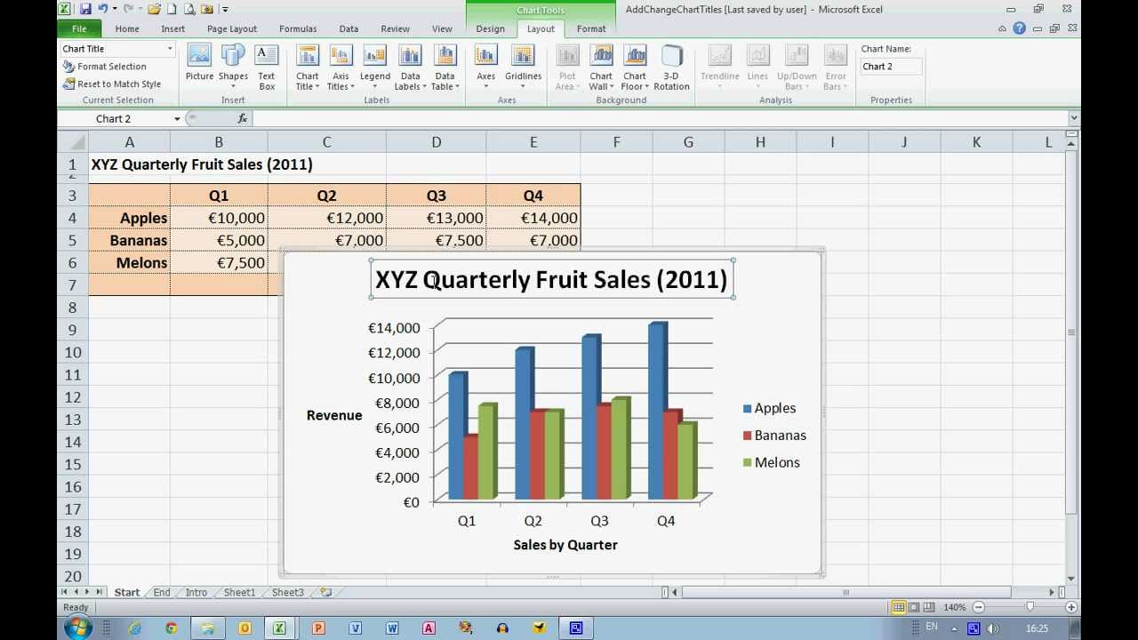
How To... Add and Change Chart Titles in Excel 2010 - YouTube
How to Create a Waterfall Chart in Excel - SpreadsheetDaddy 1. Start by selecting the data you need for your chart ( A1:B5 ). 2. Open the Insert tab. 3. Go to the Charts section and select the dropdown with the Waterfall chart option. 4. Choose the Waterfall chart. And just like that, you have your waterfall chart.
Post a Comment for "43 how to add chart labels in excel"