42 excel pivot table labels
Data Labels in Excel Pivot Chart (Detailed Analysis) 7 Suitable Examples with Data Labels in Excel Pivot Chart Considering All Factors 1. Adding Data Labels in Pivot Chart 2. Set Cell Values as Data Labels 3. Showing Percentages as Data Labels 4. Changing Appearance of Pivot Chart Labels 5. Changing Background of Data Labels 6. Dynamic Pivot Chart Data Labels with Slicers 7. How to Create Excel Pivot Table (Includes practice file) Jun 28, 2022 · The area to the left results from your selections from [1] and [2]. You’ll see that the only difference I made in the last pivot table was to drag the AGE GROUP field underneath the PRECINCT field in the Row Labels quadrant. How to Create Excel Pivot Table. There are several ways to build a pivot table.
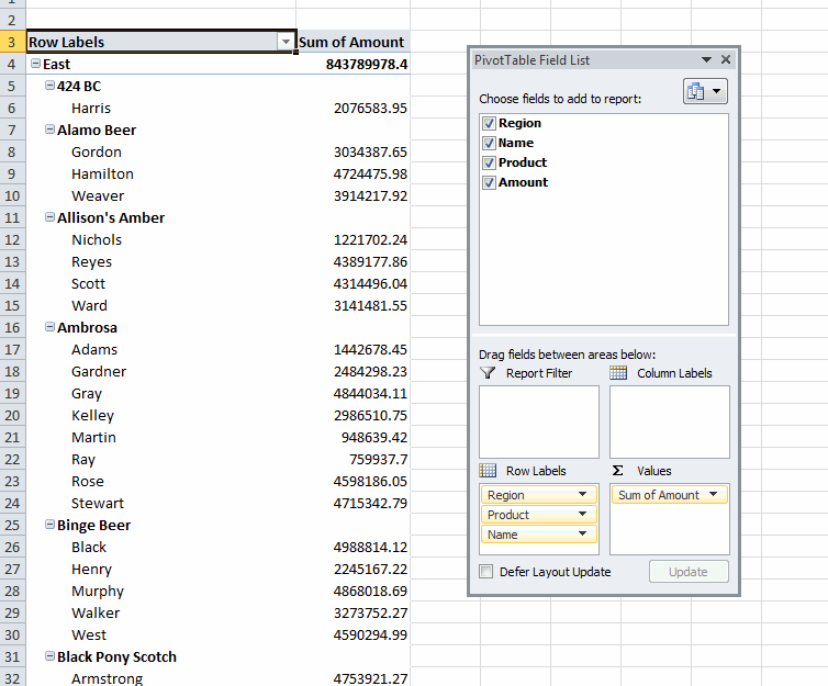
How to Create a Pivot Table in Excel - Spreadsheeto Using Pivot Table Fields. A Pivot Table ‘field’ is referred to by its header in the source data (e.g. ‘Location’) and contains the data found in that column (e.g. San Francisco). By separating data into their respective ‘fields’ for use in a Pivot Table, Excel enables its user to:

Excel pivot table labels
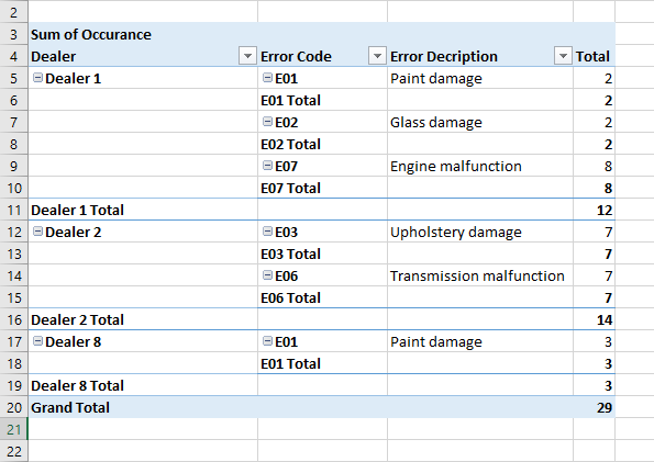
Pivot Table Row Labels In the Same Line - Beat Excel! It is a common issue for users to place multiple pivot table row labels in the same line. You may need to summarize data in multiple levels of detail while rows labels are side by side. In this post I'm going to show you how to do it. ... After creating a pivot table in Excel, you will see the row labels are listed in only one column. But, if ... Excel Pivot Table Filter and Label Formatting With Pivot charts you can copy the format of one to another by selecting the first pivot chart. Press Ctrl-C. Select the second pivot chart and press Ctrl-V. So, if you copy the pivot table and create you second pivot chart on that one, then you can copy the exact format from the first one. 0 Likes Reply Johnbda replied to Riny_van_Eekelen multiple fields as row labels on the same level in pivot table Excel ... I created a table below similar to how my data is (except with way more columns in my actual sheet). What I want to do is list all of Part A #s with the monthly volume for each, below that Part B #s with monthly volume, and below that Part C #s with monthly volume and so on, with Part A through Part E listed under the same column in the pivot.
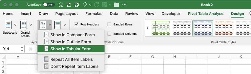
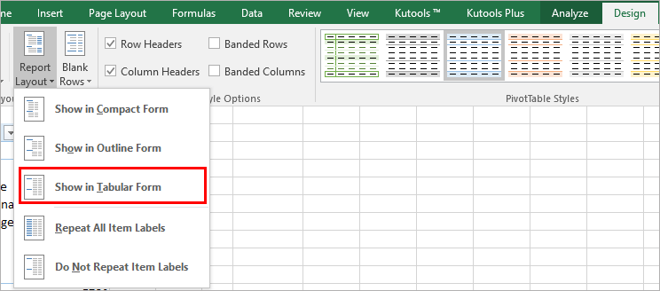
Excel pivot table labels. How to Group Data in Pivot Table (3 Simple Methods) Steps: At the very beginning, select the dataset and insert a PivotTable. Next, make sure to select the New Worksheet option and press OK. Then, group the data by going to the PivotTable Analyze tab and selecting Group Selection. In turn, the various groups appear as shown in the picture below. Sorting to your Pivot table row labels in custom order [quick tip] Add sort order column along with classification to the pivot table row labels area. Add the usual stuff to values area. Set up pivot table in tabular layout. Remove sub totals; Finally hide the column containing sort order. Your new pivot report is ready. Good news for people with Excel 2013 or above: How to Use Excel Pivot Table Label Filters - Contextures Excel Tips Right-click a cell in the pivot table, and click PivotTable Options. In the PivotTable Options dialog box, click the Totals & Filters tab In the Filters section, add a check mark to 'Allow multiple filters per field.' Click the OK button, to apply the setting and close the dialog box. Quick Way to Hide or Show Pivot Items Pivot table row labels in separate columns • AuditExcel.co.za Our preference is rather that the pivot tables are shown in tabular form (all columns separated and next to each other). You can do this by changing the report format. So when you click in the Pivot Table and click on the DESIGN tab one of the options is the Report Layout. Click on this and change it to Tabular form.
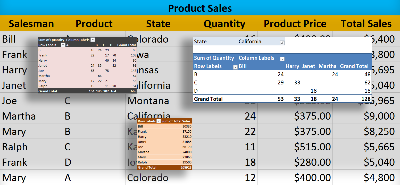
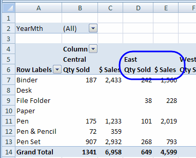
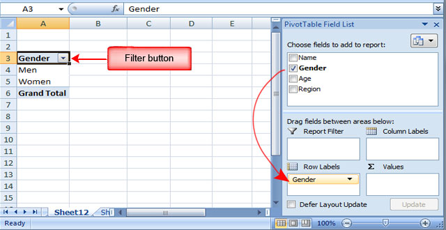
Change Blank Labels in a Pivot Table - Contextures Blog You can type any text to replace the (Blank) entry, even a space character, but you can't clear the cell and leave it empty: Select one of the Row or Column Labels that contains the text (blank). Type N/A in the cell, and then press the Enter key. Note: All other (Blank) items in that field will change to display the same text, N/A in this ... How to Use Label Filters for Text in the Pivot Table? Label Filters for Text in the Pivot Table - A Glance: You can use Row Label Filter or Column Label Filter in the pivot table to filter your required data based on the field items. If you have a huge list of data and you want to filter it based on the text string, then you can use this filter to make your work much easier. Excel Pivot values as column labels - Stack Overflow If you have Excel for Office 365 (or Excel 2021) with the FILTER function, you can use the following: Note that I used a table with structured references for the data source. This has advantages in editing the table in the future. For "pivot" header: =TRANSPOSE(SORT(UNIQUE(Table1[Country]))) For the columns: Hierarchy in excel pivot table - xchp.collegelifecoach.info The table above shows the total sales amounts for. Follow these easy steps to create an Excel pivot table, to summarize Excel data. Watch a video, try an interactive pivot, follow written steps, get free workbook. When you select a cell within the pivot table, a PivotTable Field List appears, at the right of
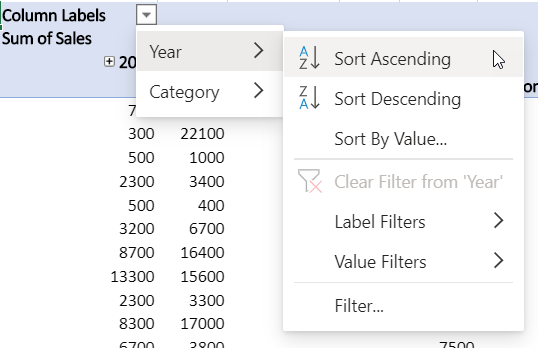
How to reset a custom pivot table row label Now go back to your Pivot and refresh it to find the Problem column and the duplicate column you just made. 5. Enter both fields into the pivot table and you will see the duplicate column has the original values while the Problem column maintains the problem labels. Monday, April 27, 2015 8:39 AM 0 Sign in to vote Excel Pivot Table Sorting Problems – Contextures Blog Sep 30, 2011 · By default, Excel’s custom lists take precedence when you’re sorting labels in a pivot table. The built-in lists and the custom lists that you create, will both affect the pivot table sorting. Fortunately, if things don’t sort the way that you need them to, you can fix the problem, by changing a pivot table setting. Pivot table row labels side by side - Excel Tutorials - OfficeTuts Excel You can copy the following table and paste it into your worksheet as Match Destination Formatting. Now, let's create a pivot table ( Insert >> Tables >> Pivot Table) and check all the values in Pivot Table Fields. Fields should look like this. Right-click inside a pivot table and choose PivotTable Options…. Check data as shown on the image below. Remove row labels from pivot table • AuditExcel.co.za Click on the Pivot table. Click on the Design tab. Click on the report layout button. Choose either the Outline Format or the Tabular format. If you like the Compact Form but want to remove 'row labels' from the Pivot Table you can also achieve it by. Clicking on the Pivot Table. Clicking on the Analyse tab.
Pivot table row labels side by side – Excel Tutorials
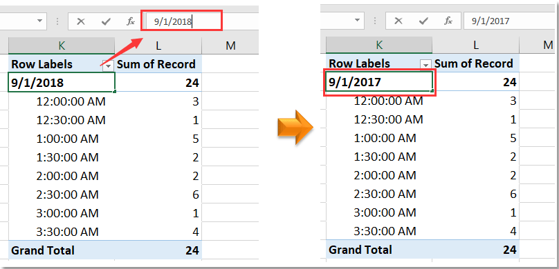
How to Move Excel Pivot Table Labels Quick Tricks - Contextures Excel Tips To move a pivot table label to a different position in the list, you can use commands in the right-click menu: Right-click on the label that you want to move Click the Move command Click one of the Move subcommands, such as Move [item name] Up The existing labels shift down, and the moved label takes its new position. Type Over Another Label

Working with Pivot Tables | Excel library | Syncfusion
How to Create Pivot Table in Excel: Beginners Tutorial - Guru99 Aug 27, 2022 · A Pivot Table is a summary of a large dataset that usually includes the total figures, average, minimum, maximum, etc. let’s say you have a sales data for different regions, with a pivot table, you can summarize the data by region and find the average sales per region, the maximum and minimum sale per region, etc. Pivot tables allow us to ...
Pivot table row labels side by side – Excel Tutorials
Repeat item labels in a PivotTable - support.microsoft.com Right-click the row or column label you want to repeat, and click Field Settings. Click the Layout & Print tab, and check the Repeat item labels box. Make sure Show item labels in tabular form is selected. Notes: When you edit any of the repeated labels, the changes you make are applied to all other cells with the same label.
How to Use a Pivot Table in Excel
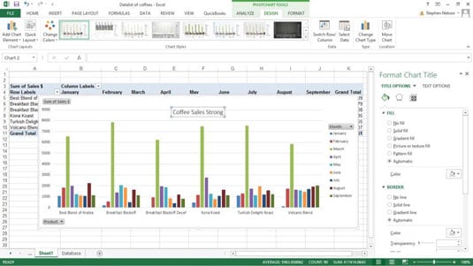
How to Customize Your Excel Pivot Chart Data Labels The Data Labels command on the Design tab's Add Chart Element menu in Excel allows you to label data markers with values from your pivot table. When you click the command button, Excel displays a menu with commands corresponding to locations for the data labels: None, Center, Left, Right, Above, and Below.
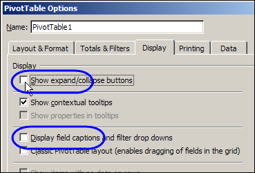
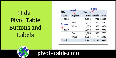
Hide Pivot Table Buttons and Labels – Contextures Blog
Hide Excel Pivot Table Buttons and Labels Jan 29, 2020 · The field labels – Year, Region, and Cat – are hidden, and they weren’t really needed. The pivot table summary is easy to understand without those labels. NOTE: You can still sort and filter the pivot fields, if you right-click on a cell, and use the commands in the pop-up menu. More Pivot Table Tips. Go to my Contextures website for more ...
How to make row labels on same line in pivot table?
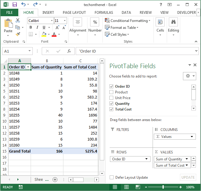
How to Set Up Excel Pivot Table - Contextures Excel Tips Aug 10, 2022 · Excel removes the field from the pivot table layout, so only the City and OrderCount fields are showing. Add More Fields . After you create your pivot table, you can add more fields, to show additional details about the data. Currently, the pivot table shows the total number of orders for each city.

How to make row labels on same line in pivot table?
How to Format Excel Pivot Table - Contextures Excel Tips Jun 22, 2022 · Video: Change Pivot Table Labels. Watch this short video tutorial to see how to make these changes to the pivot table headings and labels. Get the Sample File. No Macros: To experiment with pivot table styles and formatting, download the sample file. The zipped file is in xlsx format, and and does NOT contain any macros.

Permanently Tabulate Pivot Table Report & Repeat All Item ...
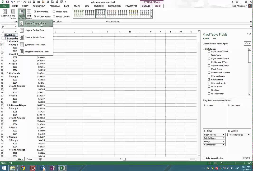
Design the layout and format of a PivotTable Change a PivotTable to compact, outline, or tabular form Change the way item labels are displayed in a layout form Change the field arrangement in a PivotTable Add fields to a PivotTable Copy fields in a PivotTable Rearrange fields in a PivotTable Remove fields from a PivotTable Change the layout of columns, rows, and subtotals
Centre Column Headings in Excel Pivot Table | Excel Pivot Tables
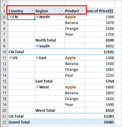
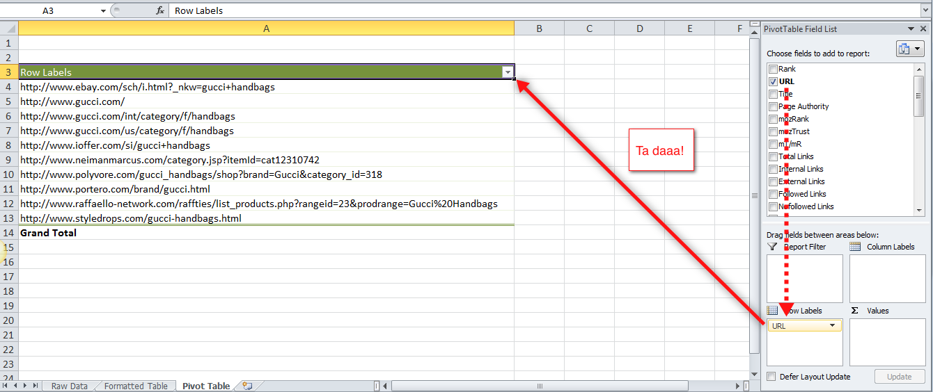
pivot table - How to extract the full row label from Excel PivotTable ... 1. I have a PivotTable in Excel with multiple layers of row filtering: Month > Region > Product (1 > EU > Dessert). When I mouse over the row, I am able to see the full row label (1 - EU - Dessert): pivot row label. I know that I can go to PivotTable Tools > Design > Report Layout > Show in Tabular Form and then Repeat All Item Labels and then ...

How to Use Label Filters for Text in the Pivot Table? - MS ...
How to Flatten Data in Excel Pivot Table? - GeeksforGeeks Select a range that you want to flatten - typically, a column of labels. Highlight the empty cells only - hit F5 (GoTo) and select Special > Blanks. Type equals (=) and then the Up Arrow to enter a formula with a direct cell reference to the first data label. Instead of hitting enter, hold down Control and hit Enter.
Design the layout and format of a PivotTable
How to make row labels on same line in pivot table? - ExtendOffice Make row labels on same line with PivotTable Options You can also go to the PivotTable Options dialog box to set an option to finish this operation. 1. Click any one cell in the pivot table, and right click to choose PivotTable Options, see screenshot: 2.
MS Excel 2013: Display the fields in the Values Section in a ...
Automatic Row And Column Pivot Table Labels - How To Excel At Excel Select the data set you want to use for your table The first thing to do is put your cursor somewhere in your data list Select the Insert Tab Hit Pivot Table icon Next select Pivot Table option Select a table or range option Select to put your Table on a New Worksheet or on the current one, for this tutorial select the first option Click Ok

Pivot Table Defaults to Count Instead of Sum & How to Fix It ...
How to rename group or row labels in Excel PivotTable? - ExtendOffice You can rename a group name in PivotTable as to retype a cell content in Excel. Click at the Group name, then go to the formula bar, type the new name for the group. Rename Row Labels name To rename Row Labels, you need to go to the Active Field textbox. 1. Click at the PivotTable, then click Analyze tab and go to the Active Field textbox. 2.

How to use another column as X axis label when you plot pivot ...
get a row label from pivot table - Microsoft Tech Community Creating PivotTable add data to data model by checking Create PivotTable and after that convert it to cube formulas. Now you may take these formulas and convert it to form you need, for example in H3 it could be =CUBEVALUE( "ThisWorkbookDataModel", CUBEMEMBER("ThisWorkbookDataModel", " [Measures].
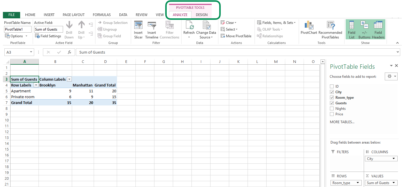
The Pivot table tools ribbon in Excel
Repeat All Item Labels In An Excel Pivot Table | MyExcelOnline DOWNLOAD EXCEL WORKBOOK. STEP 1: Click in the Pivot Table and choose PivotTable Tools > Options (Excel 2010) or Design (Excel 2013 & 2016) > Report Layouts > Show in Outline/Tabular Form STEP 2: Now to fill in the empty cells in the Row Labels you need to select PivotTable Tools > Options (Excel 2010) or Design (Excel 2013 & 2016) > Report Layouts > Repeat All Item Labels

How to Use Excel Pivot Table Label Filters
Pivot Table Row Labels - Microsoft Community If you go to PivotTable Tools > Analyze > Layout > Report Layout > Show in Tabular Form, your column headers will be used for the row labels. Every once in a while there's a sudden gust of gravity... Report abuse 1 person found this reply helpful · Was this reply helpful? Yes No A. User Replied on December 19, 2017

Fix Excel Pivot Table Missing Data Field Settings
multiple fields as row labels on the same level in pivot table Excel ... I created a table below similar to how my data is (except with way more columns in my actual sheet). What I want to do is list all of Part A #s with the monthly volume for each, below that Part B #s with monthly volume, and below that Part C #s with monthly volume and so on, with Part A through Part E listed under the same column in the pivot.
How to rename group or row labels in Excel PivotTable?
Excel Pivot Table Filter and Label Formatting With Pivot charts you can copy the format of one to another by selecting the first pivot chart. Press Ctrl-C. Select the second pivot chart and press Ctrl-V. So, if you copy the pivot table and create you second pivot chart on that one, then you can copy the exact format from the first one. 0 Likes Reply Johnbda replied to Riny_van_Eekelen
Excel 2021 (Mac) - pivot tables - "Show items labels in ...
Pivot Table Row Labels In the Same Line - Beat Excel! It is a common issue for users to place multiple pivot table row labels in the same line. You may need to summarize data in multiple levels of detail while rows labels are side by side. In this post I'm going to show you how to do it. ... After creating a pivot table in Excel, you will see the row labels are listed in only one column. But, if ...
Repeating Values in Pivot Tables – Daily Dose of Excel
Pivot Table headings that say column/ row instead of actual ...
How to Flatten and repeat Row Labels in a Pivot Table
Hide Excel Pivot Table Buttons and Labels | Excel Pivot Tables

How to Customize Your Excel Pivot Chart Data Labels - dummies

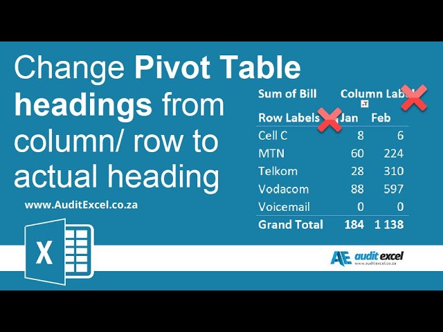
Change Pivot Table Sum of Headings and Blank Labels - YouTube

excel pivot table - multiple label filters - Stack Overflow

EXCEL: SETTING PIVOT TABLE DEFAULTS - Strategic Finance

Pivot table row labels in separate columns • AuditExcel.co.za

Repeat all item labels in Pivot Table (aka Fill in the blanks ...
How to make row labels on same line in pivot table?
How To Manage Big Data With Pivot Tables

Microsoft Excel Pivot Tables - Excel Consultant
Microsoft Excel Training in Columbus | Make Tech Easy With EasyIT

Pivot table row labels side by side – Excel Tutorials

Repeat all item labels in Pivot Table (aka Fill in the blanks ...
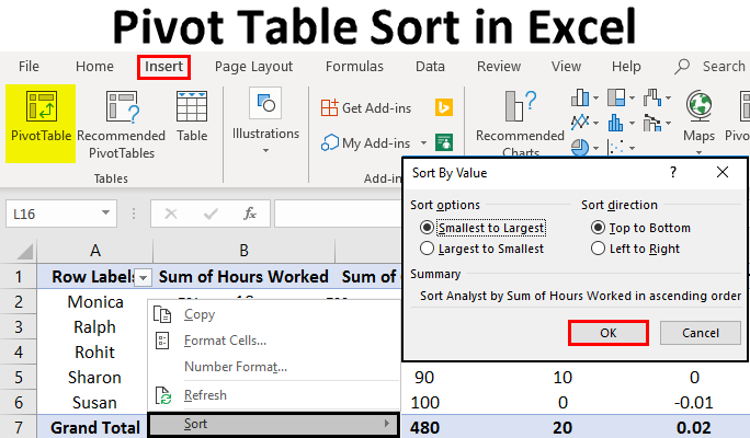
Pivot Table Sort in Excel | How to Sort Pivot Table Columns ...
Lesson 54: Pivot Table Row Labels - Swotster

Repeat item labels in a PivotTable

java - Apache POI : Excel Pivot Table - Row Label - Stack ...
How to Customize Your Excel Pivot Chart and Axis Titles - dummies

Pivot table row labels in separate columns • AuditExcel.co.za

Microsoft Excel – showing field names as headings rather than ...
Post a Comment for "42 excel pivot table labels"